Plots - powerful convenience for visualization in Julia
Author: Thomas Breloff (@tbreloff)
To get started, see the tutorial.
Almost everything in Plots is done by specifying plot attributes.
Tap into the extensive visualization functionality enabled by the Plots ecosystem, and easily build your own complex graphics components with recipes.
Intro to Plots in Julia
Data visualization has a complicated history. Plotting software makes trade-offs between features and simplicity, speed and beauty, and a static and dynamic interface. Some packages make a display and never change it, while others make updates in real-time.
Plots is a visualization interface and toolset. It sits above other backends, like GR, PythonPlot, PGFPlotsX, or Plotly, connecting commands with implementation. If one backend does not support your desired features or make the right trade-offs, you can just switch to another backend with one command. No need to change your code. No need to learn a new syntax. Plots might be the last plotting package you ever learn.
The goals with the package are:
- Powerful. Do more with less. Complex visualizations become easy.
- Intuitive. Start generating plots without reading volumes of documentation. Commands should "just work."
- Concise. Less code means fewer mistakes and more efficient development and analysis.
- Flexible. Produce your favorite plots from your favorite package, only quicker and simpler.
- Consistent. Don't commit to one graphics package. Use the same code and access the strengths of all backends.
- Lightweight. Very few dependencies, since backends are loaded and initialized dynamically.
- Smart. It's not quite AGI, but Plots should figure out what you want it to do... not just what you tell it.
Use the preprocessing pipeline in Plots to describe your visualization completely before it calls the backend code. This preprocessing maintains modularity and allows for efficient separation of front end code, algorithms, and backend graphics.
Please add wishlist items, bugs, or any other comments/questions to the issues list, and join the conversation on zulip.
Nevertheless, extreme configurability is not a goal of Plots. If you require a rather specific plotting feature, feel free to request it. However, do understand that Plots has to implement the feature across all backends which might be challenging due some backends' limitations.
Simple is Beautiful
Lorenz Attractor
using Plots
# define the Lorenz attractor
Base.@kwdef mutable struct Lorenz
    dt::Float64 = 0.02
    σ::Float64 = 10
    ρ::Float64 = 28
    β::Float64 = 8/3
    x::Float64 = 1
    y::Float64 = 1
    z::Float64 = 1
end

function step!(l::Lorenz)
    dx = l.σ * (l.y - l.x)
    dy = l.x * (l.ρ - l.z) - l.y
    dz = l.x * l.y - l.β * l.z
    l.x += l.dt * dx
    l.y += l.dt * dy
    l.z += l.dt * dz
end

attractor = Lorenz()

# initialize a 3D plot with 1 empty series
plt = plot3d(
    1,
    xlim = (-30, 30),
    ylim = (-30, 30),
    zlim = (0, 60),
    title = "Lorenz Attractor",
    legend = false,
    marker = 2,
)

# build an animated gif by pushing new points to the plot, saving every 10th frame
@gif for i=1:1500
    step!(attractor)
    push!(plt, attractor.x, attractor.y, attractor.z)
end every 10
Make some waves
using Plots
default(legend = false)
x = y = range(-5, 5, length = 40)
zs = zeros(0, 40)
n = 100

@gif for i in range(0, stop = 2π, length = n)
    f(x, y) = sin(x + 10sin(i)) + cos(y)

    # create a plot with 3 subplots and a custom layout
    l = @layout [a{0.7w} b; c{0.2h}]
    p = plot(x, y, f, st = [:surface, :contourf], layout = l)

    # induce a slight oscillating camera angle sweep, in degrees (azimuth, altitude)
    plot!(p[1], camera = (10 * (1 + cos(i)), 40))

    # add a tracking line
    fixed_x = zeros(40)
    z = map(f, fixed_x, y)
    plot!(p[1], fixed_x, y, z, line = (:black, 5, 0.2))
    vline!(p[2], [0], line = (:black, 5))

    # add to and show the tracked values over time
    global zs = vcat(zs, z')
    plot!(p[3], zs, alpha = 0.2, palette = cgrad(:blues).colors)
end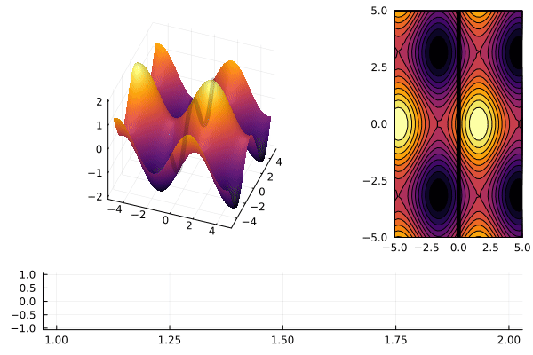
Iris Dataset
# load a dataset
using RDatasets
iris = dataset("datasets", "iris");

# load the StatsPlots recipes (for DataFrames) available via:
# Pkg.add("StatsPlots")
using StatsPlots

# Scatter plot with some custom settings
@df iris scatter(
    :SepalLength,
    :SepalWidth,
    group = :Species,
    title = "My awesome plot",
    xlabel = "Length",
    ylabel = "Width",
    m = (0.5, [:cross :hex :star7], 12),
    bg = RGB(0.2, 0.2, 0.2)
)